PhD Research

1. Molecular structure prediction as an NP-hard problem

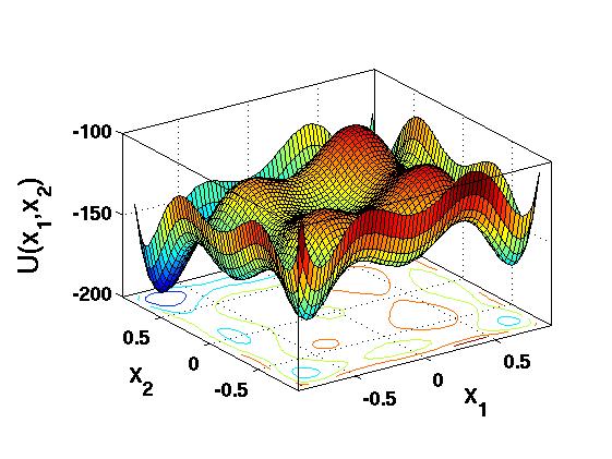
Much of theoretical chemistry and computational biology reduces to one hard question: given a system of atoms, what is its lowest-energy configuration? Proteins, atomic clusters and spin glasses are studied as points in a high-dimensional configuration space moving on a potential energy surface (PES). Near the global minimum of a funnel-like landscape the entropic contribution is often negligible, so finding the equilibrium structure amounts to finding the global minimum of the PES ^[1].

This is genuinely hard. The number of local minima grows exponentially with system size, and deciding the global non-negativity of a general polynomial of degree four or higher is NP-hard. Conventional methods — Monte Carlo, simulated annealing, genetic algorithms — sample the surface but can never certify that the global minimum has been found; exhaustive sampling scales exponentially.

2. Sum-of-squares optimisation

Sum-of-squares (SOS) optimisation, developed by Parrilo ^[2] and Lasserre ^[3], takes a different route entirely: rather than sampling, it produces a certified lower bound by convex optimisation. To minimise a polynomial $U(\mathbf{x})$ we seek the largest scalar $\lambda$ that stays below it everywhere:

$$U(\mathbf{x}) - \lambda \ge 0, \qquad \lambda \in \mathbb{R}, \quad \forall\, \mathbf{x} \in \mathbb{R}^n.$$

Deciding that non-negativity is exactly the NP-hard step. The key idea is to relax it: instead of requiring $U(\mathbf{x}) - \lambda \ge 0$, require that it be a sum of squares,

$$f^{\,\mathrm{sos}} = \sum_{i=1}^{r} \big(p_i(\mathbf{x})\big)^2 \;\ge\; 0,$$

which is automatically non-negative. Remarkably, a great many non-negative polynomials are also sums of squares, so this is a tight relaxation. Crucially, a polynomial is SOS if and only if it admits a Gram-matrix factorisation

$$U(\mathbf{x}) - \lambda = \mathbf{z}^{\mathsf T} Q\, \mathbf{z},$$

where $\mathbf{z}$ is the vector of monomials and $Q \succeq 0$ is positive semidefinite. The coefficients of $U$ impose linear constraints on $Q$, so finding the best bound becomes a semidefinite programme (SDP):

$$\begin{aligned}\text{maximise}\quad & \lambda \\ \text{subject to}\quad & Q \succeq 0,\\ & \operatorname{Tr}(A_i Q) = b_i,\quad i = 1,\dots,m.\end{aligned}$$

SDPs are convex and solvable in polynomial time by interior-point methods. This buys three things sampling cannot: (i) the problem is lifted from coordinate space into the space of coefficients and solved as a convex programme; (ii) the original function is never sampled or deformed; and (iii) duality furnishes a certificate of optimality. The bound is guaranteed, and can be tightened systematically at the cost of more computation. Every SDP comes paired with a dual programme, and for the SOS bound the dual is the moment relaxation of Lasserre ^[3]. Where the primal searches over Gram matrices $Q$, the dual searches over moments $y_\alpha$ — surrogates for the averages $\langle \mathbf{x}^{\alpha} \rangle$ of the monomials in $\mathbf{z}$. Replacing each monomial of $U$ by its moment linearises the objective, and the one nonlinear demand — that the moments come from a genuine point — is relaxed to requiring only that the moment matrix $M(y)$, with entries $M(y)_{\alpha\beta} = y_{\alpha+\beta}$, be positive semidefinite:

$$\begin{aligned}\text{minimise}\quad & \sum_{\alpha} U_\alpha\, y_\alpha \\ \text{subject to}\quad & y_{0} = 1,\\ & M(y) \succeq 0.\end{aligned}$$

The two programmes squeeze the true minimum from the same side and, at optimum, meet exactly:

$$\lambda^{\star} \;=\; \sum_{\alpha} U_\alpha\, y^{\star}_\alpha \;\le\; \min_{\mathbf{x}} U(\mathbf{x}).$$

Weak duality is what turns a sum-of-squares decomposition into an instantly checkable proof: to confirm that $\lambda$ is a valid lower bound, one need only verify the algebraic identity $U(\mathbf{x}) - \lambda = \mathbf{z}^{\mathsf T} Q\, \mathbf{z}$ with $Q \succeq 0$ — no search, no sampling. Strong duality (which holds here under a Slater condition) closes the gap, so the best SOS bound $\lambda^{\star}$ equals the optimal moment value. The certificate of optimality then lives in the rank of $M(y^{\star})$: when it is rank one, the moment matrix factors as $M(y^{\star}) = \mathbf{z}(\mathbf{x}^{\star})\,\mathbf{z}(\mathbf{x}^{\star})^{\mathsf T}$ for a genuine point $\mathbf{x}^{\star}$, whose moments give $U(\mathbf{x}^{\star}) = \lambda^{\star}$. The lower bound is attained — which proves $\mathbf{x}^{\star}$ is a global minimiser and that the relaxation was exact. The two halves interlock: the SOS decomposition proves nothing can beat $\lambda^{\star}$, while the rank-one moment solution exhibits a point that achieves it.

So far $U$ has been minimised over all of $\mathbb{R}^n$, but a molecule lives on a constrained surface — fixed bond lengths, excluded volume, geometric closure. These enter as polynomial inequalities $g_j(\mathbf{x}) \ge 0$ that carve out a feasible region

$$K = \{\,\mathbf{x} \in \mathbb{R}^n : g_j(\mathbf{x}) \ge 0,\ \ j = 1,\dots,\ell\,\},$$

on which $U(\mathbf{x}) - \lambda$ need only be non-negative — not everywhere. The bridge from this geometric condition back to an SOS programme is a cornerstone of real algebraic geometry, the Positivstellensatz (Stengle, Putinar): for a bounded $K$, any polynomial positive on it can be written as

$$U(\mathbf{x}) - \lambda = \sigma_0(\mathbf{x}) + \sum_{j=1}^{\ell} \sigma_j(\mathbf{x})\, g_j(\mathbf{x}), \qquad \sigma_0,\ \sigma_j \ \text{sums of squares}.$$

This can be considerd as a Lagrangian in monomial space. The SOS polynomials $\sigma_j(\mathbf{x})$ play exactly the role of Lagrange multipliers — but where classical duality offers only non-negative scalars $\mu_j \ge 0$ in $U - \sum_j \mu_j\, g_j$, here the multipliers are non-negative polynomials, free to vary across configuration space and weight each constraint precisely where it binds. Since each $\sigma_j$ is a sum of squares it is non-negative, so every term $\sigma_j g_j$ is non-negative on $K$ and the identity is itself a proof that $U \ge \lambda$ there.

Fixing the degree of the multipliers turns the search for the $\sigma_j$ back into a semidefinite programme, and raising that degree performs a systematic lifting: the products $\sigma_j(\mathbf{x})\, g_j(\mathbf{x})$ introduce higher-order monomials as fresh coordinates, embedding the original non-convex surface in a higher-dimensional space where it straightens into a convex spectrahedron. Each added degree is a tighter convex relaxation, and the sequence — the Lasserre hierarchy ^[3] — converges to the true constrained minimum. The intractable, non-convex geometry of the molecule is thereby traded for a nested family of convex problems a solver can actually handle.

In practice the SOS programme is not assembled by hand. The polynomial is handed to SOSTOOLS ^[9], a MATLAB toolbox that parses the sum-of-squares constraints and automatically builds the underlying SDP; that SDP is then solved by SeDuMi ^[10], an efficient primal–dual interior-point solver for symmetric cones. SOSTOOLS recovers the Gram matrix $Q$ and the sum-of-squares decomposition from the solver output, so the certified lower bound — and its proof — come straight out of the pipeline.

3. Applying SOS to molecular structure — parametrising the Amber force field

SOS needs a polynomial objective, but a classical force field is not polynomial. The Amber94 force field ^[4] writes the energy as a sum of bonded and non-bonded terms:

$$\begin{aligned} E = {}& \sum_{\text{bonds}} K_r (r - r_{eq})^2 + \sum_{\text{angles}} K_\theta (\theta - \theta_{eq})^2 + \sum_{\text{dihedrals}} \frac{V_n}{2}\big[1 + \cos(n\phi - \gamma)\big] \\ & {}+ \sum_{i<j} \left[ \frac{A_{ij}}{r_{ij}^{12}} - \frac{B_{ij}}{r_{ij}^{6}} + \frac{q_i q_j}{\varepsilon\, r_{ij}} \right]. \end{aligned}$$

The harmonic bond and angle terms are already quadratic, but the torsional cosine series and the non-bonded terms (in $r^{-12}$, $r^{-6}$ and $r^{-1}$) are not polynomials. The work therefore maps each Amber term into polynomial form — fitting polynomials to the torsional functional and to the van der Waals and Coulombic contributions as functions of the relevant internal coordinate (e.g. the dihedral angle $\phi$), with changes of variable for the rational terms. Taking ethane (C₂H₆) as a case study, the full potential was recast as a polynomial and its global minimum certified with the SOS/SDP machinery above — demonstrated first on model potentials with deliberately pathological landscapes, then on this real molecular system ^[5].

4. Coarse-grained molecular dynamics via second-order cone programming

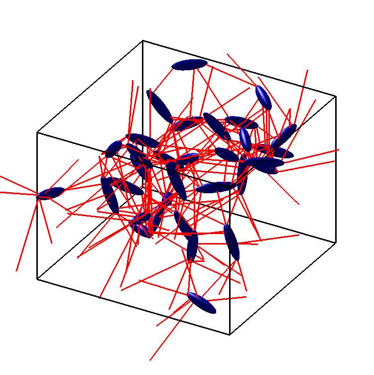
The second strand coarse-grains molecules as ellipsoids — single-site anisotropic particles in the spirit of the Gay–Berne potential ^[6]. An ellipsoid is the set $E = \{\, \mathbf{x}\in\mathbb{R}^3 : (\mathbf{x}-\mathbf{c})^{\mathsf T} A\,(\mathbf{x}-\mathbf{c}) \le 1 \,\}$ with $A \succ 0$. Realistic anisotropic potentials depend on the minimum distance between two such particles ^[7] — but that distance is itself an optimisation problem:

$$d(E_1, E_2) = \min_{\mathbf{x}\in E_1,\ \mathbf{y}\in E_2} \lVert \mathbf{x} - \mathbf{y} \rVert_2.$$

This is convex and can be cast as a second-order cone programme (SOCP), exploiting the same equivalence between a sum-of-squares polynomial and the quadratic form defining the ellipsoid. The programme we built (MOLSOCP) solves this conic programme — via the MOSEK conic solver ^[11] — at every step of the molecular-dynamics integration to obtain the exact minimum-distance vector $\mathbf{a}-\mathbf{b}$ between neighbouring particles, and from it the inter-particle force and torque. To our knowledge this was the first coarse-grained MD in which the true minimum distance — not an approximation — is used at each step ^[8].

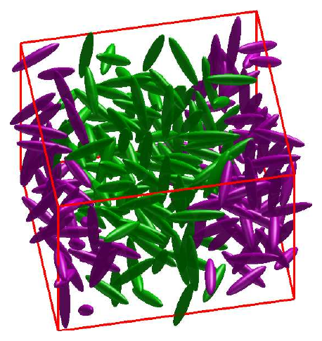
Inside the simulation

Each ellipsoid is a rigid body with six degrees of freedom — three translational, three rotational — with orientation tracked by quaternions to avoid the singularities that Euler angles suffer. Translational motion follows Newton’s equations and rotational motion Euler’s equations in the body-fixed frame; the run is in reduced Lennard–Jones units with periodic boundaries and the minimum-image convention. Each timestep the programme (i) builds an interaction list of pairs within a centre-to-centre cutoff; (ii) solves the SOCP for every listed pair to get the exact minimum-distance vector; (iii) evaluates a shifted Lennard–Jones force along that vector — shifted so it goes smoothly to zero at the cutoff, for energy conservation and stability — together with the resulting torque about the centre of mass,

$$\boldsymbol{\tau} = \mathbf{f}_{ij} \times \mathbf{a},$$

where $\mathbf{a}$ is the vector to the contact point; and (iv) integrates the equations of motion and accumulates statistics (kinetic, potential and total energy).

In short

The thread is a single, unconventional idea: reframe hard, non-convex problems in chemistry — global structure prediction, and anisotropic coarse-grained interactions — as convex optimisation (semidefinite and second-order cone programmes), gaining guarantees and efficiency that sampling-based methods cannot offer.

Relevance to AI

Modern machine learning is, at its core, large-scale non-convex optimisation built on heavy linear algebra, and the themes here map directly onto current AI research: convex relaxations that turn intractable non-convex problems into tractable ones with provable guarantees (now used, for example, in the certified verification and robustness analysis of neural networks); semidefinite programming and the positive-semidefinite cone (linear algebra in one of its most powerful forms); and the spectral and matrix machinery that underpins both. In fact the very semidefinite / sum-of-squares relaxations at the heart of my thesis are now an active tool in AI research in their own right — for example, certifying that no adversarial perturbation within a given budget can fool a trained neural network, which turns robustness verification into exactly the kind of convex relaxation of an intractable non-convex problem studied here ^[12].

There is an even more direct link. The structure-prediction problem at the heart of my thesis — finding a molecule's lowest-energy configuration on a rugged, high-dimensional energy landscape — is, at protein scale, precisely the protein-folding problem that AlphaFold so dramatically solved ^[13]. Where my PhD attacked small model systems by explicit energy minimisation through convex relaxations, AlphaFold reached the same goal from the opposite direction — learning the sequence-to-structure map directly from data — a vivid sign that the very class of problem I worked on is where modern AI has had some of its greatest scientific impact.

References

1. D. J. Wales, Energy Landscapes. Cambridge University Press, 2003.
2. P. A. Parrilo, “Semidefinite programming relaxations for semialgebraic problems,” Mathematical Programming 96 (2003) 293–320.
3. J. B. Lasserre, “Global optimization with polynomials and the problem of moments,” SIAM J. Optimization 11 (2001) 796–817.
4. W. D. Cornell et al., “A second generation force field for the simulation of proteins, nucleic acids, and organic molecules,” J. Am. Chem. Soc. 117 (1995) 5179–5197.
5. M. G. Burke and S. N. Yaliraki, “Exploring model energy and geometry surfaces using sum of squares decompositions,” J. Chem. Theory Comput. 2 (2006) 575–587.
6. J. G. Gay and B. J. Berne, “Modification of the overlap potential to mimic a linear site–site potential,” J. Chem. Phys. 74 (1981) 3316–3319.
7. L. Paramonov and S. N. Yaliraki, “The directional contact distance of two ellipsoids: coarse-grained potentials for anisotropic interactions,” J. Chem. Phys. 123 (2005) 194111.
8. L. Paramonov, M. G. Burke and S. N. Yaliraki, “Coarse-Grained Dynamics of Anisotropic Systems,” in G. A. Voth (Ed.), Coarse-Graining of Condensed Phase and Biomolecular Systems, CRC Press, 2009.
9. S. Prajna, A. Papachristodoulou and P. A. Parrilo, SOSTOOLS: Sum of Squares Optimization Toolbox for MATLAB, 2002–2004.
10. J. F. Sturm, “Using SeDuMi 1.02, a MATLAB toolbox for optimization over symmetric cones,” Optimization Methods and Software 11 (1999) 625–653.
11. MOSEK ApS, The MOSEK optimization software.
12. A. Raghunathan, J. Steinhardt and P. Liang, “Semidefinite relaxations for certifying robustness to adversarial examples,” Advances in Neural Information Processing Systems (NeurIPS) 31 (2018).
13. J. Jumper, R. Evans, A. Pritzel et al., “Highly accurate protein structure prediction with AlphaFold,” Nature 596 (2021) 583–589.